djtaylor.me

Monte carlo confidence intervals

Consider the following setup: you have a continuous probability distribution $F$ conditioned on an unknown parameter $T$. You have an observation $obs$ that's been sampled from $F$, and you want to find, say, the 50% confidence interval for the hidden parameter $T$.

To make matters better, the observations have a fairly natural measure on them $M$ (e.g. you're dealing with a probability distribution over the reals or euclidean space or something), and $\frac{dF}{dM}$ is "continuous enough" and doesn't have any "flat section." And the set that $T$ comes from has some natural measure on it too, and that nudging $T$ a bit doesn't change $F$ too much.

Also you have the ability to, given a value of $T$, sample from $F$ fairly easily. And that you have the ability to accurately calculate (or, later on in the post, calculate an estimator for) $\frac{dF}{dM}(x \vert T)$.

deep breath

If all those conditions are satisfied, then it's possible to calculate pointwise estimates of confidence intervals. What I mean by that, is that there exists a Monte-Carlo style algorithm that will, given an input value of $T$, will produce a estimated "yes, this $T$ is in the 50% (or whatever) CI" or "no, this $T$ is NOT in the 50% (or whatever) CI." Then many subsequent iterations of the algorithm can be merged to get a more accurate estimate.

The thing

In this post we're going to be taking inspiration from the Fisher exact method for generating $p$-confidence intervals, where $p$ is your confidence level, like 50% or 75% or whatever. This is my definition:

Fix some value of $T$. Let $S$ be the smallest set of observations, according to $M$, such that $F(S \vert T) \ge p$. If $obs \in S$, then $T$ is in the $p$-confidence set interval.

In this definition, the $p$-confidence interval isn't actually an interval at all. But that's okay, I'm calling it an interval because the words "confidence interval" are too ingrained in my mind to start calling them anything different.

Also, in this definition, $S$ exists and is unique. Actually it isn't. Two different values of $S$ will agree almost everywhere, relative to $M$. For the following paragraphs I will be assuming that any annoyances like isolated points and boundaries have been removed from $S$. I don't know, if you care about this kind of thing, figure it out yourself. I'm not your mother.

One important fact about this definition is that there exists a value, call it $L$, such that any $x$ that satisfies $L \lt \frac{dF}{dM}(x \vert T)$ is also in $S$, and any $x$ for which it greater than or equal is not in $S$. If your $S$ violates this, then it's not the smallest $S$.

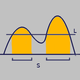
Another way to say it is that if your $x$ is in the $S$ for this $T$'s $p$-confidence interval, then $\frac{dF}{dM}(x \vert T)$ is going to be greater than $(1 - p)$ percentage of values of $\frac{dF}{dM}(y \vert T)$, for $y$'s drawn randomly according to $F$.

So the route to a Monte Carlo confidence interval becomes clear:

// Generating the samples
input obs

samples = empty array;
loop some number of times {
	T = generate a value of T uniformly according to its measure mentioned earlier;
	x = generate a sample of F given T;

	p1 = calculate dF/dM (x | T);
	p2 = calculate dF/dM (obs | T);

	if (p1 < p2) {
		push (T, true) into samples;
	} else {
		push (T, false) into samples;
	}
}

// Using the samples
input T, p

look around the area in the neighborhood of the value of T, and see if there are any samples that exist there;
denom = total number of samples in that region;
num = number of samples in that region with the value true;
if (denom == 0) {
	indeterminate;
} else if ((1 - p) < num / denom) {
	T is in p-confidence interval;
} else {
	T is NOT in p-confidence interval;
}

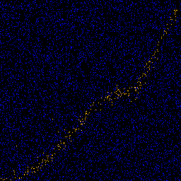
This process will generated images that look something like this:

These estimators of being inside/outside the confidence interval are NOT unbiased. A small amount of bias is introduced when two $T$'s share their samples.

Example 1

To start off I'm going to be using a simple example just to verify that everything is working as intended. The setup:

$F$ is a triangular distribution with a width of 0.5, centered on $T$. $M$ and the topology on the $T$'s are just normal ones on the real numbers.

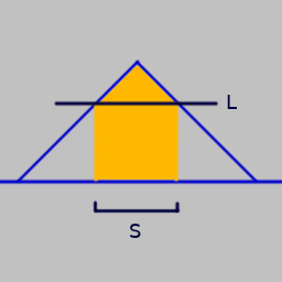
Since the distribution doesn't change with $T$, only translates, it's easy to derive different confidence intervals. For an observation of 0.6, the 50% CI for $T$ is about $(obs - 0.073, obs + 0.073)$, the 75% CI is $(obs - \frac{1}{8}, obs + \frac{1}{8})$, and the 95% CI is about $(obs - 0.19, obs + 0.19)$. So $(0.527, 0.673)$, $(0.475, 0.725)$, and $(0.41, 0.79)$ respectively.

Here I did things a little differently. Instead doing a certain number of samples and then doing a sort of windowed blur, in these examples I directly drew 256 samples per pixel and did the calculation with a window width of 1 pixel. And I think the results match up with theory!

Example 2

In the introduction, I said that one necessary condition is that $\frac{dF}{dM}$ is continuous. It's pretty easy to come up with discrete distributions for which the above algorithm fails miserably. But as long as your discrete distribution is "continuous enough", like a binomial distribution with lots of trials, you shouldn't run into too much trouble.

Also in the above, calculating $\frac{dF}{dM}(x \vert T)$ exactly was required. But oftentimes it's only possible to compute an estimate of the probability density.

Just using the an estimator of the density of course adds quite a bit of bias. Because if $g$ is an estimator of $\frac{dF}{dM}(obs \vert T)$, and $h_o$ is an estimator of $\frac{dF}{dM}(o \vert T)$, then

$$\begin{align}& \int \chi\left(\frac{dF}{dM}(obs \vert T) - \frac{dF}{dM}(o \vert T)\right) dM(o) \\= & \int \chi\left(\int g(y_1) dy_1 - \int h_o(y_2) dy_2\right) dM(o) \\\ne & \iiint \chi\left(g(y_1) - h_o(y_2)\right) \, dy_1 \, dy_2 \, dM(o)\end{align}$$

Two easy mitigations I show below are supersampling and importance sampling. There is also a potential option that I haven't tried yet that I think will be mostly applicable to progressive/online algorithms, where you have some trade off between sharing samples for the purpose of determining confidence interval inclusion/exclusion, and sharing samples for the purpose of calculating better estimates of the densities.

Unfortunately I couldn't think of an easy example to demonstrate the validity of these modifications. The example I'm going with instead is:

I'm going to be generating confidence intervals for the CDF of a distribution given some data. The $T$ in this case is 2-dimensional plane of (observations, CDF probability value) pairs. And $\frac{dF}{dM}$, given $T$, is the probability of seeing that data given $T$. So for example, the observed data set has 100 elements in it, and if the $T$ chosen is (50, 0.25), and if 30% of the actual data is less than 50, then $\frac{dF}{dM}(data \vert T) = \sum \tbinom{100}{30} 0.25^{30} 0.75^{70}$. However, despite the fact that it's not that hard to calculated $\frac{dF}{dM}$ directly, I'm going to be estimating and using importance sampling for demonstration purposes.

To make it more clear, here's some code:

generate_sample(r, trials) {
	int ret = 0;
	for (int i = 0; i < trials; ++i) {
		if (nrand() < r) {
			ret += 1;
		}
	}
	return ret;
}

estimate_prob(obs, r, trials) {
	prob = 0;
	// Super sampling
	for (int ss = 0; ss < NUM_SUPER_SAMPLES; ++ss) {
		// Importance sampling
		weight = 1;
		track = 0;
		for (int i = 0; i < trials; ++i) {
			if (obs == (track + (trials - 1))) {
				track += 1;
				weight *= r;
			} else if (obs == track) {
				track += 0;
				weight *= (1 - r);
			} else if (nrand() < r) {
				track += 1;
			} else {
				track += 0;
			}
		}
		prob += weight / NUM_SUPER_SAMPLES;
	}
	return prob;
}

// Generating the samples
input data

samples = empty array;
loop some number of times {
	T = generate a (x on the horizontal axis of the CDF, real number r in [0,1] to be interpreted as the value of the CDF at x) pair according to their measures;

	empirical_obs = number of data points less than x;
	adversary_obs = generate_sample(r, number of data points);

	p1 = estimate_prob(adversary_obs, r, number of data points);
	p2 = estimate_prob(empiricle_obs, r, number of data points);

	if (p1 < p2) {
		push (T, true) into samples;
	} else {
		push (T, false) into samples;
	}
}

// Using the samples is the same

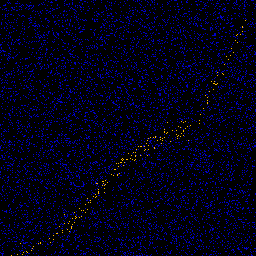
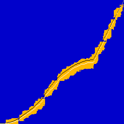
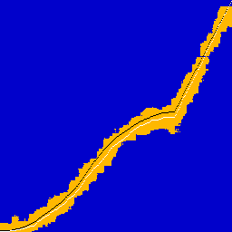
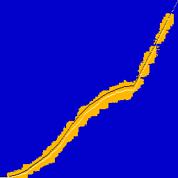
And some pictures. Black overlay is ground truth CDF, white is the CDF of the observed 1024 data points.

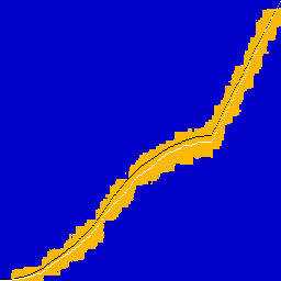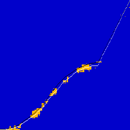
Note how, for low supersampling, the confidence set is visibly larger, and there are a number of spurious data points far away from the main cluster.

The end

Other things I want to do with this:

• Write up another post applying it to the two problems I originally came up with this for: object tracking and undoing a probability density convolution.
• Come up with examples demonstrating consistency of the CI estimator with the modifications.
• As you can probably see, the efficiency of this estimator leaves something to be desired. 8k samples were thrown at the CDF example, and the vast majority of them were obvious falses. Come up with an importance sample strategy for this as well.
• One interesting thing about this algorithm is that you can adjust the $p$ level without having to recalculate the samples. So I need to make a javascript demonstration of this that has full interactibility.